Prediction Variance & Scaled Prediction Variance
Prediction Variance
In addition to coefficient estimation, one key reason we conduct experiments is to predict future performance of a system. Prediction variance describes the error involved with making a prediction using a regression model. Consider an operational test that consists of runs and factors. The corresponding first order regression model is
Scaled Prediction Variance
Scaled Prediction Variance (SPV), on the other hand, normalizes the prediction variance by
 Figure 1
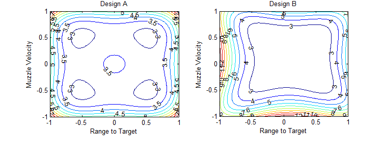 Careful inspection of Figure 1 shows that while Design B has a larger region with the minimal SPV (less than 3.5), a greater portion of the design space for Design A has an SPV less than 4.0. Meanwhile, the SPV near the extremes is much greater for Design B. Based on these observations, Design A is the preferred experimental design for the limited 10 shots.
In this example, it is reasonable to characterize SPV because it is a two-dimensional problem. In cases where there are more than two factors, when the characterization is not straight forward, there are different types of summarizing graphs that can be used to compare experimental designs, such as the Fraction of Design Space plot.
Careful inspection of Figure 1 shows that while Design B has a larger region with the minimal SPV (less than 3.5), a greater portion of the design space for Design A has an SPV less than 4.0. Meanwhile, the SPV near the extremes is much greater for Design B. Based on these observations, Design A is the preferred experimental design for the limited 10 shots.
In this example, it is reasonable to characterize SPV because it is a two-dimensional problem. In cases where there are more than two factors, when the characterization is not straight forward, there are different types of summarizing graphs that can be used to compare experimental designs, such as the Fraction of Design Space plot.