Combining Information: Reliability for the Stryker Family of Vehicles
By:
On:
Reliability is an essential element in assessing the operational suitability of Department of Defense (DoD) weapon systems. It takes a prominent role in both the design and the analysis of operational tests. In the current era of reduced budgets and increased reliability requirements, it is challenging to verify reliability requirements in a single test. However, there has been an increased interest in capturing data consistently across all stages of testing, and these data can be intelligently combined using statistical methods.
This case study describes the benefits of using parametric statistical models to combine information from the developmental and operational test phases for the Stryker family of vehicles (FOV). Both frequentist and Bayesian inference techniques are employed, and they are compared and contrasted to illustrate different statistical methods for combining information.
Scenario and Test Goal
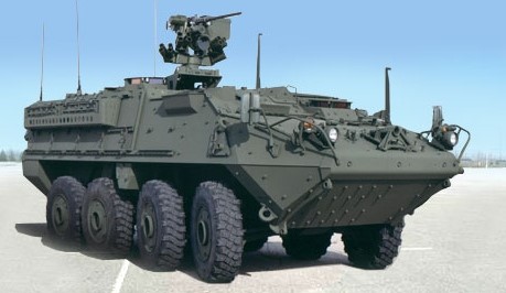
The Stryker is a family of wheeled armored combat vehicles built for the U.S. Army. The FOV includes ten separate system configurations, with two main versions of the vehicle under which these ten systems can be organized: the Infantry Carrier Vehicle (ICV) and the Mobile Gun System (MGS). The ICV is the focus of this case study. It serves as the base vehicle for the eight remaining system configurations: Antitank Guided Missile Vehicle (ATGMV), Commander’s Vehicle (CV), Engineer Squad Vehicle (ESV), Fire Support Vehicle (FSV), Medical Evacuation Vehicle (MEV), Mortar Carrier Vehicle (MCV), Reconnaissance Vehicle (RV) and the Nuclear, Biological and Chemical Reconnaissance Vehicle (NBC RV). The purpose of this case study is to combine information from the different system configurations during the Developmental Test (DT) and Operational Test (OT) in order to obtain reliability estimates. To accomplish this goal, frequentist and Bayesian inference techniques to combine information through the use of formal statistical models are explored.
Figure 1. The Infantry Carrier Vehicle (ICV) serves as the base vehicle for eight additional system configurations
Method
Data
The data used in this case study come from the Stryker FOV developmental and operational testing in 2003. The NBC RV system configuration was excluded from this case study because it was on a different acquisition timeline, and therefore does not have data from the same tests as the other variants.
The Army reliability requirement for the Stryker is that the vehicle have a mean of 1,000 miles between System Abort (SA), where an SA is defined by a failure that results in the loss or degradation of an essential function that renders the system unable to enter service or causes immediate removal from service. Table 1 provides a summary of the Stryker FOV reliability data by test phase (DT or OT) and vehicle variant (system configuration). Included in this table are the total number of miles driven, the number of SAs, and the number of right censored observations. Right censoring occurs when the testing of the vehicle was terminated before an SA was observed. Of the 263 observations recorded, 199 of these were SA failures (131 SAs in DT and 68 SAs in OT) and the remaining 64 observations were right censored (12 in DT and 52 in OT).
Table 1. Stryker 2003 Data Summary by Vehicle Variant and Test Phase
Vehicle Variant
Developmental Test
Operational Test
TotalMiles
SystemAborts
RightCensored
TotalMiles
SystemAborts
RightCensored
ATGMV
30086
17
1
10334
12
9
CV
24160
11
2
8494
1
6
ESV
25095
35
2
3771
13
3
FSV
24385
11
2
2306
1
2
ICV
61623
39
3
29982
35
23
MCV
3702
7
1
4521
4
4
MEV
--
--
--
1967
0
2
RV
23742
11
1
5374
2
3
Total
192793
131
12
66749
68
52
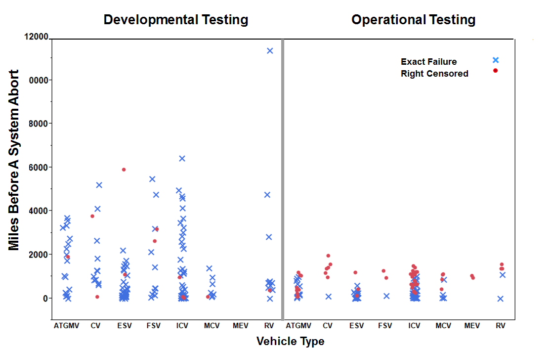
As can be seen in Table 1 and Figure 2, there was a higher rate of censoring in OT because of the limited test time (two weeks) and larger numbers of test assets. This higher rate of censoring also affects the spread of the data; there is more variability in the DT failure distances than there is in the OT failure distances (see Figure 2).
Figure 2. Scatter plot of the Stryker 2003 data grouped by test phase and vehicle type
A limitation in these data is that there are nine instances in which the vehicle’s SA failure mileage was recorded as a zero. These nine responses were spread over the different vehicle variants and the two test phases, and they are the result of finding another SA failure during the repair of a primary SA failure. To account for these special cases in the data, two separate entries were recorded: the first entry records the exact mileage for the initial SA that stopped the vehicle, while the second entry records the discovered SA and uses the response value of zero in the mileage column.
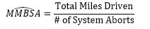
Current DoD Analysis
A standard reliability analysis employed by the DoD test community considers each test phase (and each vehicle type in this case) independently and uses the exponential distribution to model the miles (or time) between SAs. The reliability of the Stryker is expressed in terms of the mean miles between an SA (MMBSA), and can be estimated as
Statistical Models for Combining DT and OT Data
Instead of considering the DT and OT phases, and the vehicle variants independently of each other, this case study aims to improve on this current reliability analysis by using parametric statistical models to formally combine the data and make inference. Figure 3 shows a comparison of the distribution of the vehicle failure miles (t) across all vehicle variants and test phases to both the exponential distribution and the Weibull distribution – two common distributions for modeling lifetime data. The Weibull distribution appears to be a better fit to the data, as the data points are closer to a straight line in the probability plot. Therefore, it is assumed the data follows a Weibull distribution.
Figure 3. Exponential (left) and Weibull (right) probability plots.
For the frequentist analysis, a Weibull regression model was used to combine the Stryker FOV data, treating test phase and all vehicle variants as explanatory variables so that individual reliability estimates for each of the vehicles within each test phase could be estimated. The MEV data were removed because there were just two right censored observations. The model fitted was the following:
Equation 1
for i = 1, 2, 3, ..., 263, the observed data points. The indicator variables in this expression were coded as
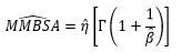
Maximization of the total likelihood was needed in order to obtain [latex]\widehat{MMBSA}[/latex]. For that, the cdf and pdf of the Weibull distribution, as well as an indicator [latex]\delta_i[/latex] were used ([latex]\delta_i = 1[/latex] if [latex]t_i[/latex] is an exact observation, and [latex]\delta_i = 0[/latex] if [latex]t_i[/latex] is a right censored observation). The maximum likelihood estimate for MMBSA is
where [latex]\beta[/latex] is the shape parameter of the Weibull distribution and assumed to be constant, and [latex]\Gamma[/latex] is the gamma function. The MMBSA estimates for each vehicle variant in both the DT and OT phases can be calculated by replacing [latex]\hat{\eta}[/latex] with its estimated expression given in Equation 1.
Bayesian hierarchical modeling also provides a rigorous way to combine information from multiple sources and different types of information. The following model specification was used to model the failure miles (t)
A multiplicative model structure was chosen specifically because it is analogous to the Weibull regression model defined in Equation 1. That is, the shift in the scale parameter from the DT to OT phase is represented by [latex]\delta[/latex].
An immediate advantage of using this type of model is that a reliability estimate for the MEV can now be obtained. This estimate is driven by the information available for the seven other vehicles. A hierarchical prior for [latex]\eta_j [/latex] can be specified using the gamma distribution.
Inferences for this multiplicative model are made by using the joint posterior distribution, which is proportional to the product of likelihood and priors. By defining the Bayesian model in this way, we are starting with by vague information (diffuse priors) about the parameters of interest and then update this beliefs with the information from the data that we collected.
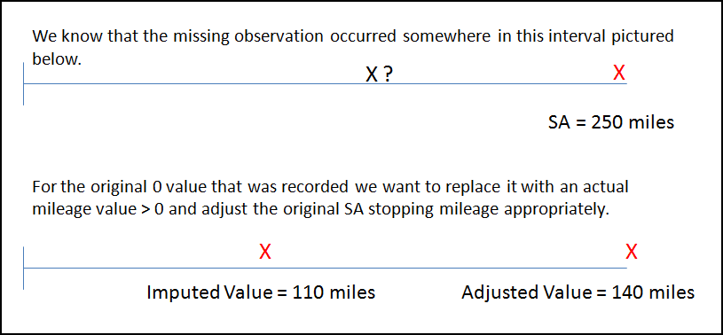
Imputing Missing data
Remember that there were nine of the SA failure miles recorded as zero, and it is known that the failure occurred in the range between the last failure and the current failure under investigation. A possible solution for this is to treat these responses as missing values and impute plausible values for [latex]t_{missing}[/latex] to complete the dataset. To avoid duplicating these miles in the total likelihood, the initial SA stopping mileage has to be corrected (see Figure 4 for an example). For the frequentist model, multiple imputation was used as a solution for missing data. In the Bayesian analysis, the following relationship was used
where the Weibull distribution is truncated at the original SA mileage.
Figure 4. Correcting for missing data - example
Results
The results of these analyses are presented, compared and contrasted in this section. Table 2 illustrates the results using OT data only (current DoD analysis), the frequentist Weibull regression analysis, and the Bayesian analysis. The first column lists the vehicle variants under consideration, the second column shows the estimate based on the exponential distribution and its exact confidence intervals using the OT data only. The next two columns show the results using the Weibull regression analysis and its Wald confidence intervals for each test phase. Finally, the MMBSA estimate using the Bayesian analysis and the respective credible intervals are shown.
Table 2. MMBSA estimates and intervals (V2)
Vehicle Variant
OT only*
Weibull regression analysis**
Bayesian analysis***
DT
OT
DT
OT
ATGMV
861 (493, 1667)
1715 (864, 2566)
1313 (584, 2042)
1872 (1137, 3009)
1541 (870, 2649)
CV
8494 (1525, 335495)
3737 (920, 6553)
2861 (556, 5166)
3231 (1677, 6136)
2664 (1291, 5346)
ESV
290 (170, 545)
626 (391, 861)
479 (241, 717)
733 (475, 1126)
608 (344, 1043)
FSV
2306 (414, 91082)
2571 (670, 4472)
1968 (342, 3595)
2552 (1330, 4769)
2114 (994, 4247)
ICV
857 (616, 1230)
1501 (982, 2020)
1149 (704, 1595)
1588 (1107, 2255)
1302 (864, 1960)
MC
1130 (441, 4148)
1015 (200, 1831)
777 (159, 1395)
1434 (621, 2856)
1175 (504, 2412)
MEV§
-- (657, --)
--
--
3084 (929, 8735)
2529 (751, 7245)
RV
2687 (743, 22187)
2695 (766, 4623)
2063 (473, 3653)
2580 (1360, 4793)
2130 (1038, 4185)
*MMBSA estimate based on the exponential distribution with exact confidence intervals.
**MMBSA estimate based on the frequentist Weibull regression analysis with Wald confidence intervals.
***MMBSA estimate and credible intervals based on the Bayesian analysis.
§There were only two right censored observations for MEV. Therefore, the OT only analysis shows a one-sided lower confidence bound and no point estimate, and the data was removed for the Weibull (frequentist) regression analysis.
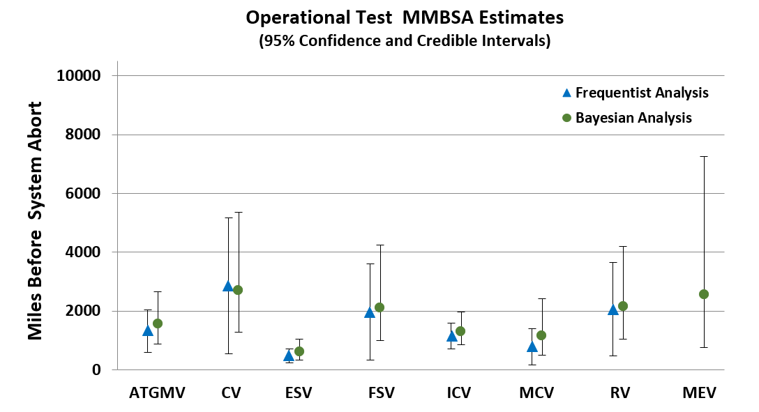
Notice how in Table 2 the CV on the OT only analysis stands out as potentially having an optimistically high MMBSA, considering that it was based on six censored observations and no individual vehicle traveled more than 2,000 miles in OT. Additionally, if we use the simple exponential estimate of the MMBSA in DT (results not shown), we find that the MMBSA was less than 2,200 miles. It is highly unlikely that we would see such a large improvement in the reliability between late DT and OT because no major changes were made to the system configuration. For the MEV, it was only possible to obtain a one-sided lower interval when using the OT data only, and no results could be obtained when using the frequentist analysis. However, it is possible to obtain a point estimate and a lower and upper bounds when using the Bayesian analysis (Table 2 and Figure 5). On the other hand, one of the advantages of the frequentist analysis is that it is available in many standard statistical packages. Also, the frequentist analysis and the current DoD analysis (OT data only) are easier to implement than the Bayesian analysis. There are statistical software that will allow you to use Bayesian analyses which require some background knowledge and coding skills.
Figure 5. A comparison of the OT MMBSA vehicle variant estimates for the frequentist analysis and Bayesian analysis using the Weibull distribution.
Although the Weibull distribution provides a better fit to the data than the exponential distribution, it may still be reasonable to use the exponential distribution, especially for inference on the means. Figure 6 compares the results of the current DoD analysis, which includes only data from the OT, to the frequentist and Bayesian analysis methods described in this paper using the exponential distribution (β=1). Notice that using a statistical model to account for changes in test phase and vehicle variant has a large practical impact on the reliability results.
The model-based analyses also improve the precision of the interval estimates (confidence and credible intervals) of system reliability for the vehicles with a small number of failures (CV, FSV, MEV and RV) by leveraging the failure information from the other variants and developmental testing. Notice that the Bayesian and frequentist model-based approaches give similar results. However, remember that we were able to obtain point estimates and intervals for MEV with the Bayesian approach, and not with the frequentist one.
Figure 6. A comparison of the Operational Test MMBSA Vehicle Variant Estimates for the Current Analysis, Frequentist Analysis and Bayesian Analysis using the exponential distribution.


 Maximization of the total likelihood was needed in order to obtain [latex]\widehat{MMBSA}[/latex]. For that, the cdf and pdf of the Weibull distribution, as well as an indicator [latex]\delta_i[/latex] were used ([latex]\delta_i = 1[/latex] if [latex]t_i[/latex] is an exact observation, and [latex]\delta_i = 0[/latex] if [latex]t_i[/latex] is a right censored observation). The maximum likelihood estimate for MMBSA is
 where [latex]\beta[/latex] is the shape parameter of the Weibull distribution and assumed to be constant, and [latex]\Gamma[/latex] is the gamma function. The MMBSA estimates for each vehicle variant in both the DT and OT phases can be calculated by replacing [latex]\hat{\eta}[/latex] with its estimated expression given in Equation 1.
Bayesian hierarchical modeling also provides a rigorous way to combine information from multiple sources and different types of information. The following model specification was used to model the failure miles (t)
where [latex]\beta[/latex] is the shape parameter of the Weibull distribution and assumed to be constant, and [latex]\Gamma[/latex] is the gamma function. The MMBSA estimates for each vehicle variant in both the DT and OT phases can be calculated by replacing [latex]\hat{\eta}[/latex] with its estimated expression given in Equation 1.
Bayesian hierarchical modeling also provides a rigorous way to combine information from multiple sources and different types of information. The following model specification was used to model the failure miles (t)
 A multiplicative model structure was chosen specifically because it is analogous to the Weibull regression model defined in Equation 1. That is, the shift in the scale parameter from the DT to OT phase is represented by [latex]\delta[/latex].
An immediate advantage of using this type of model is that a reliability estimate for the MEV can now be obtained. This estimate is driven by the information available for the seven other vehicles. A hierarchical prior for [latex]\eta_j [/latex] can be specified using the gamma distribution.
A multiplicative model structure was chosen specifically because it is analogous to the Weibull regression model defined in Equation 1. That is, the shift in the scale parameter from the DT to OT phase is represented by [latex]\delta[/latex].
An immediate advantage of using this type of model is that a reliability estimate for the MEV can now be obtained. This estimate is driven by the information available for the seven other vehicles. A hierarchical prior for [latex]\eta_j [/latex] can be specified using the gamma distribution.
 where the Weibull distribution is truncated at the original SA mileage.