Bayesian intervals: incorporating prior information
Many techniques used to analyze test results come from what is known as a "frequentist" framework, in which terms such as "hypothesis testing," "confidence intervals," and "p-values" appear often. The frequentist framework is built around the concept of long-run probability. That is, probability is conceptualized as the proportion of times an event will occur over a long sequence of events. Increasingly, a Bayesian approach to modeling is being considered as a powerful alternative to this frequentist framework. For an overview of Bayesian analysis, see our introductory material. The Bayesian framework is characterized by many strengths, including the ability to incorporate information from across multiple samples or from previously existing information. This may supplement limited data, which, in turn, allows for increased precision and reduced costs. Specifically, the Bayesian framework allows for the introduction of a “prior” parameter that uses information from prior studies or from prior knowledge. The three steps of the process we will illustrate are:- Construct a prior from previously existing information (e.g., old test data from a similar system)
- Construct the likelihood from your collected test data (e.g., your sample data)
- Estimate posterior distribution using Bayes’ theorem (put all of the pieces together)
Example: Missile launch system
Suppose we have a missile launch system, and we are interested in the probability of obtaining a successful launch. The missile is launched nine times. We observe six successful launches and three failed launches. These nine observation points constitute our test data. Now, for a new missile launch system, a point estimate of our probability of success would be the number of successes divided by the number of attempts, , or 0.67. This value provides our point estimate for the probability of a successful launch.How would a frequentist approach proceed?
In a frequentist approach, we could construct a 95% confidence interval around this point estimate (0.67) and provide an interval estimate of the long-run probability of a successful launch. We could construct this interval using a normal approximation binomial confidence interval. The normal approximation is one of several options for computing a confidence interval around a binomial proportion. To do this, we would take the expression for a normal approximation binomial confidence interval and fill it in with relevant information from our example: [latex]\hat{p} \pm z_{\alpha = .05}\sqrt{\frac{\hat{p}(1-\hat{p})}{n}}[/latex] [latex]\frac{6}{9} \pm z_{\alpha = .05}\sqrt{\frac{\frac{6}{9}(1-\frac{6}{9})}{9}}[/latex] where \(\hat{p}\) is our point estimate, \(n\) is our number of total launches, and \(\pm 1.96\) is the value of the \(z\) distribution at \(\alpha = .025\) and \(\alpha = .975\) . Plugging in these numbers yields a confidence interval of \(.39 \leq p \leq .98\).How is this frequentist interval interpreted?
When interpreting this confidence interval, it is important to keep in mind how probability is interpreted in the frequentist framework. This interval can be interpreted as follows: if the test were repeated an infinite number of times and we constructed a confidence interval each time, then 95% of the confidence intervals will contain the true probability of a successful launch. That is, the frequentist approach cannot tell us the probability that this specific interval contains the true probability of a successful launch. However, if we were to proceed in a Bayesian framework, we could obtain exactly this type of interval. That is, we could make a direct probability statement regarding the certainty that our constructed interval contains the true probability of a successful launch, a statement that is likely of strong interest to a decision maker. In doing so, we may also draw on a strength of the Bayesian framework; namely, we may incorporate prior information. We demonstrate this below.How would a Bayesian approach proceed?
Suppose that, in conjunction with the aforementioned test data, a researcher has access to historical data of a similar missile launch system. In these historical data, testers launched six missiles; they observed five successful launches and one failed launch. These historical data are valuable, especially in testing environments where sample size may be limited due to cost or resources. We can incorporate these historical data in the form of a prior distribution, reflecting prior knowledge we have regarding the value of our parameter (here, the probability of success). For variables whose values range between 0 and 1 (such as probability values), the beta distribution is a natural choice to represent our prior information. Additionally, the beta distribution is the "conjugate prior" for the binomial distribution. By “conjugate prior,” we mean that the beta prior distribution combines with the likelihood function to produce a posterior with the same form as the prior. In plain terms, the beta distribution mathematically “gets along” with the binomial distribution. We can represent our prior in the form \(\theta^a(1-\theta)^b\), where \(\theta\) is the probability of success, \(a\) is our historical number of successful launches, and \(b\) is our historical number of failed launches. It is helpful to note that the probability of success for a single launch can be thought of as a Bernoulli trial (like a coin flip) and is a function of \(\theta\). Thus the probability of the success of a single launch can be expressed as: [latex]p(y|\theta) = \theta^y(1-\theta)^{1-y}[/latex] where \(y\) is 0 or 1, representing either a failed or successful launch, respectively. It is helpful to note that this expression simplifies to \(p(y|\theta)\) when \(y = 1\). Using to represent the set of all outcomes of our test data \({y_i}\) we can express the likelihood as [latex]L(\theta) = \theta^x(1-\theta)^{N-x}[/latex] A close inspection shows that our likelihood function, \(\theta^x(1-\theta)^{N-x}\) is in a similar form as our prior distribution, \(\theta^a(1-\theta)^b\). The prior and likelihood can then be incorporated using Bayes’ theorem. By substituting our likelihood (from our test data) and our beta prior distribution (from our historical data) into Bayes’ theorem, we can obtain a posterior probability of a successful launch. The full steps of substitution and simplification are not shown here. When our prior distribution is in the form \(beta(\theta|a,b)\) and our data contain \(x\) successful launches out of \(N\) attempts, then we can express our posterior as [latex]beta(\theta|x+a, N-x+b)[/latex] [latex]beta(\theta|6+5,9-6+1)[/latex] [latex]beta(11,4)[/latex] We can visually represent these pieces of information.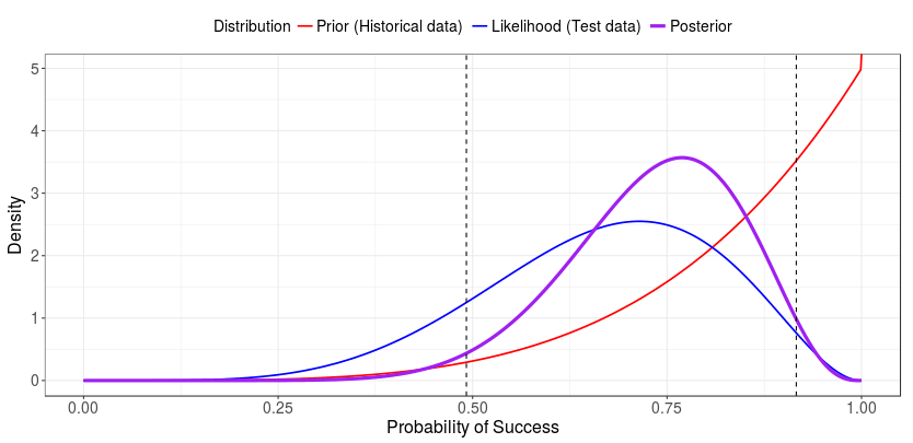 Here, the prior distribution is represented with a solid red line, the likelihood is represented with a solid blue line, and the posterior distribution is represented with a solid purple line.
From the posterior distribution, we can compute a 95% credible interval. Specifically, we compute the 95% posterior central interval, one form of Bayesian credible interval. We compute this interval by obtaining the 2.5th and 97.5th percentile of the posterior distribution; it is represented above by dashed gray lines. We can see here that the posterior distribution is influenced by the prior and likelihood distributions.
The posterior mean is equal to \((x+a)/(n+a+b)\), or 0.733. The 95% credible interval, (0.49, 0.92), means that the probability that \(\theta\) is in the interval of (0.49, 0.92) is 0.95.
Note the intuitive nature of this interpretation compared to the frequentist confidence interval. That is, we do not have to make any statements regarding long-run probabilities; instead, we can make a direct probability statement. This is because the Bayesian framework treats parameters as random, not fixed, variables. Note also that in this case, our credible interval is narrower than our confidence interval, in part due to the incorporation of prior data. In this case, the incorporation of prior data allowed us more precision in our estimate of \(\theta\). Had our prior distribution disagreed greatly with the distribution we saw in our data, this interval would have been wider, reflecting more uncertainty. Further, had our prior data come from a much larger sample, the prior would have had a much larger influence on the shape of the posterior distribution.
For more information on Bayesian credible intervals, see the Wikipedia page. Want to compute a Bayesian credible interval and plot all of the pieces yourself? Try our Shiny app for computing Bayesian credible intervals.
[1] Note that these z values come from the standard normal distribution.
Here, the prior distribution is represented with a solid red line, the likelihood is represented with a solid blue line, and the posterior distribution is represented with a solid purple line.
From the posterior distribution, we can compute a 95% credible interval. Specifically, we compute the 95% posterior central interval, one form of Bayesian credible interval. We compute this interval by obtaining the 2.5th and 97.5th percentile of the posterior distribution; it is represented above by dashed gray lines. We can see here that the posterior distribution is influenced by the prior and likelihood distributions.
The posterior mean is equal to \((x+a)/(n+a+b)\), or 0.733. The 95% credible interval, (0.49, 0.92), means that the probability that \(\theta\) is in the interval of (0.49, 0.92) is 0.95.
Note the intuitive nature of this interpretation compared to the frequentist confidence interval. That is, we do not have to make any statements regarding long-run probabilities; instead, we can make a direct probability statement. This is because the Bayesian framework treats parameters as random, not fixed, variables. Note also that in this case, our credible interval is narrower than our confidence interval, in part due to the incorporation of prior data. In this case, the incorporation of prior data allowed us more precision in our estimate of \(\theta\). Had our prior distribution disagreed greatly with the distribution we saw in our data, this interval would have been wider, reflecting more uncertainty. Further, had our prior data come from a much larger sample, the prior would have had a much larger influence on the shape of the posterior distribution.
For more information on Bayesian credible intervals, see the Wikipedia page. Want to compute a Bayesian credible interval and plot all of the pieces yourself? Try our Shiny app for computing Bayesian credible intervals.
[1] Note that these z values come from the standard normal distribution. 